
joshua angrist shares the nobel prize!
Some of you may have heard the news already, but if you haven’t: on Monday, Joshua Angrist, the Ford International Professor of Economics at MIT, won the Nobel Prize in Economics (officially, the 2021 Sveriges Riksbank Prize in Economic Sciences in Memory of Alfred Nobel)! He shares the award with two others: David Card (of UC Berkeley) and Guido Imbens (of the Stanford Graduate School of Business).
Officially, this prize was awarded to Card “for his empirical contributions to labour01 economics”, and jointly to Angrist and Imbens for “for their methodological contributions to the analysis of causal relationships”. There’s a lot of depth behind both of these contributions, and as someone who blogs and is very interested in labor economics and methods of causal inference,02 I feel almost obligated to blog about what exactly this Nobel Prize was for.
Much research that happens in economics is very different from what you might see in AP Micro or AP Macro. Economists study the economy very broadly: central banking and interest rates and stock markets, yes, but also kidney exchange “markets” without money, creating environmental policy with respect to climate change, health insurance, and so much more.
Many economists do work that relates to causal relationships.03 In essence, what we’d like to understand is the chains of cause-and-effect in the economy. Many questions are of the form of “What is the impact of X policy on Y?” where X and Y can be, quite literally, anything:
- the effect of unemployment insurance on the amount of time unemployed
- the effect of free pre-school on schooling and wages later in life
- the effect of carbon-tax policies on emissions
- the effect of free trade on economic growth
- the effect of immigration on local employment and wages.
The rest of this blog is going to talk about how economists try to answer these kinds of questions, and some of the cooler findings that Angrist, Card, and Imbens have found.
Many scientists — biologists, chemists, physicists, and so on — have a cut-and-dry, formulaic way of approaching questions of causality: e.g., does my new vaccine help prevent malaria infections? Their experiments go something like this:
- Randomly assign patients (or whatever you’re studying) to a “treatment” group and some to a “control” group.
- For those in the treatment group, give them your intervention (in this case, your vaccine).04
- Because the treatment and control group were assigned randomly, your treatment effect is just the difference between the treatment group’s outcomes and the control group’s outcomes.
Now, why does step 3 work for computing the causal impact of our intervention? If I wanted to understand the impact of my vaccine, my ideal experiment would be to take a person, give them the vaccine, and see if they ever develop measles. Then, I’d like to take the exact same person, and see what happens to them without the vaccine. Finally, I’d compare the two numbers (also replicating the process with many, many other people), and that would give me the causal effect.
But there is a problem here: I do not have a time machine to go back and study the same person twice: once with the vaccine and once without. This is often called “unobservable counterfactuals”: we cannot know something (unobservable) that didn’t actually happen (a counterfactual).
Instead, scientists use the randomization process described above: and the “random” part of this is important. When you randomly assign people to treatment and control groups, you shouldn’t expect there to be much of a difference in the characteristics between the two groups. While each individual person might have differing susceptibility to malaria (their overall health, they might live in a more malaria-prone region, etc.), if the population you study is large enough, the law of large numbers says that any differences between the two groups will become insignificant. This is what makes the third step work: the data from the control group will be identical (in expectation) to what the treatment group would have looked had they not been treated.
Unfortunately, economists cannot do this so easily. Randomly assigning some people to get unemployment insurance and others to have none would be ethically and morally questionable. For trade policy, you’d need to get governments from across the world to let economics “flip a coin” to determine their trade embargoes and tariffs, which will never happen. Of course, there are some times when economists can randomize interventions; that was, in fact, the subject of the 2019 Nobel Prize partially awarded to MIT Professors Esther Duflo and Abhijit Banerjee, who have used randomized control trials to evaluate many anti-poverty programs. But such trials aren’t feasible for many other things that we’d like to study.
Take schooling, for example. We might be interested in how going to school impacts people’s incomes. We might get a graph like this:
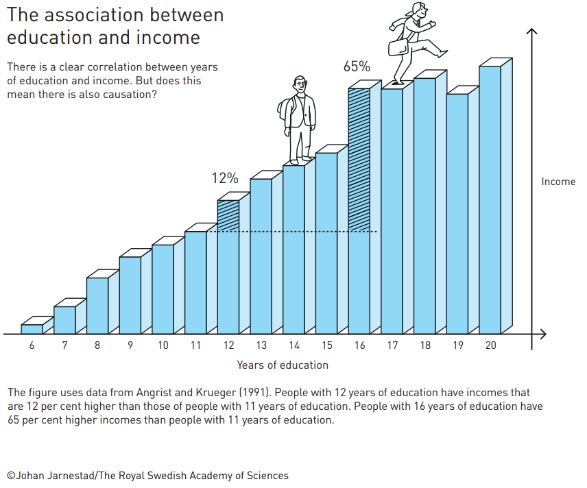
source: link
At first, the data might seem convincing: people with more education get higher wages, so education causes income to go up! But, there’s a catch: people self-select into education. What if the people who choose to go to college might have been better at studying when they left high school, a trait that would have granted them higher wages even if they didn’t go to college? If this is the case, we might be mistaking the impact of ability on income for the impact of school on income. In essence, correlation is not causation. Fundamentally, the people who choose to go to school differ from those who don’t in ways beyond having a diploma or not. We don’t have a good “control” group like scientists do for malaria drug trials.
Or take the minimum wage, for example. We might be interested in understanding if raising the minimum wage affects employment. Some argue that when the minimum wage goes up, businesses can’t afford to hire as many workers, and so fewer people will be working. But data on the minimum wage and employment across all 50 states won’t be able to tell us whether this relationship is causal, because not every state is equally comparable. So how can we do it?
The state of New Jersey increased its minimum wage by 80 cents in 1992. Suppose our graph of employment looked something like this. What could we conclude?
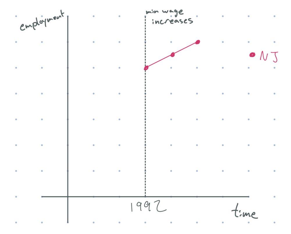
figure 1: after 1992 (minimum wage increase), new jersey employment goes up. (assume the dot on the line is data from before the policy had impacts.)
If you answered nothing, you’re completely right. While employment does seem to increase after the policy was implemented, we don’t know if this was a causal impact. Maybe employment would have increased even without the policy. Or maybe employment would have skyrocketed in absence of the wage change, but the minimum wage stunted growth. We don’t know. If we were to simply look at data from pre- and post-policy, and tried to interpret it causally, we would need to assume that there was no time effect. And that probably isn’t true: we might be in an economic boom, the federal government may have changed labor laws, there may have been new developments in firm technology, …
How might we deal with time effect? Say that we had data from a neighboring state — like Pennsylvania — that had no such minimum wage increase, and we observed the following . What could we learn from this graph?

figure 2: after 1992 (minimum wage increase), new jersey employment goes up, and employment in pennsylvania goes up by the same amount
“Aha!”, you might say. “We can see that employment in New Jersey is going upwards after the minimum wage change, but at the same rate as Pennsylvania, which had no such wage change; as such, the policy had no impact on employment at all!” In math terms, we’d be saying that the effect of the wage increase is
(Change in NJ line over time)–(Change in PA line over time)(Δ)
This is almost, almost, right — but there’s just one problem. If this is truly the effect, it would assume that the time trend in untreated Pennsylvania is the same time trend that New Jersey had if it were untreated. Is that true?
It turns out there’s no way to verify this claim by looking at data; like in the measles vaccine example above, the time trend for New Jersey in the absence of the minimum wage change is an unobservable counterfactual. Instead, this is an assumption called “parallel trends”, so named because if Pennsylvania and New Jersey did have the same time effect, in the absence of the policy, the graphs of Pennsylvania and New Jersey would indeed be parallel.
What we can do is provide suggestive evidence that the parallel trends assumption holds. Consider the graph below, which includes data from many time periods before the minimum wage increase.
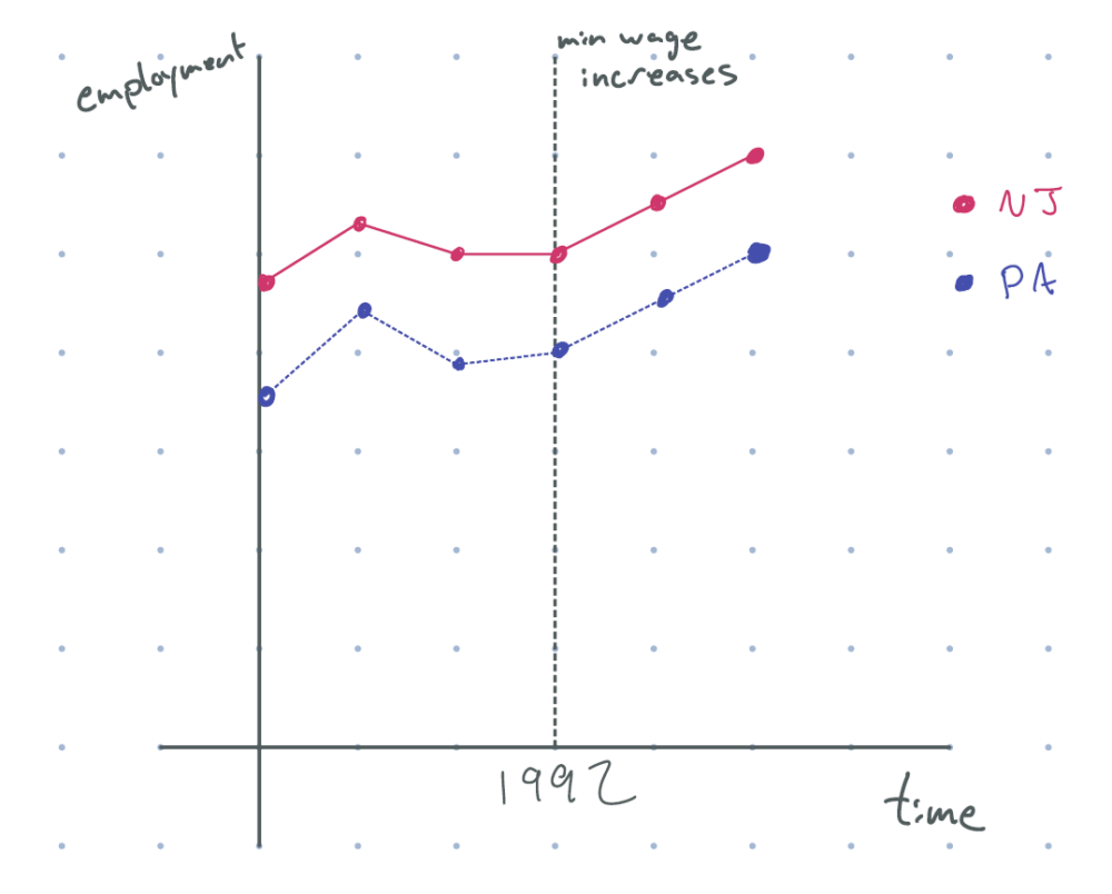
figure 3: after 1992 (minimum wage increase), new jersey employment goes up, and employment in pennsylvania goes up by the same amount, with parallel pre-trends
Now, this is convincing. The paths of Pennsylvania and New Jersey looked roughly parallel before the wage change, which means that they probably would have had a similar trend in the absence of the wage change. But, because the two states actually looked parallel after the wage change, we can conclude that the minimum wage had no effect on employment in New Jersey.
This method is known as difference-in-differences, or D-in-D, named because the equation labeled (Δ) is a difference of two differences. This exact estimator was used by Card and Krueger (who passed away in 2019, but likely would have shared the Nobel Prize if not) in this exact setting, in a paper from 1994 titled “Minimum Wages and Employment: A Case Study of the Fast-Food Industry in New Jersey and Pennsylvania”.
Card and Krueger examined the impact of an 80-cent increase in the minimum wage on food-service employment05 in New Jersey when compared to the employment in eastern Pennsylvania.06 The wage hike is an example of a natural experiment (or quasi-experiment) that economists use to understand how the world works. Unlike scientists running real experiments, natural experiments happen when something happens in the world (like a policy implementation) that we can use to analyze the mechanisms that underlie the world around us.
Another very classic example of a D-in-D paper, cited by the Nobel Prize Committee, is Card (1990), “The Impact of the Mariel Boatlift on the Miami Labor Market”. This paper uses the impact of immigration from Cuba on wages in Miami (when compared to some other cities in the US), finding that immigration had effectively zero impact on locals’ wages.
I’ve talked about two papers so far (and will talk about more below); but before going on, I’d like to emphasize that each paper I cite is just one paper in a body of evidence. One paper’s conclusion is not the “truth” in economics. Quasi-experiments in different settings might find different effects. Newer methodologies might refine the results. In addition, these papers aren’t perfect; they’re over 20 years old, and people have pointed out many, many flaws with them. But these papers are important, and Nobel Prize-worthy, because they helped start an era in economics where people think very deeply about answering these questions with “good” estimators.
Of course, I’ve only talked about David Card’s research here; there’s still another half of the Nobel Prize that I haven’t gotten to here (including Josh Angrist’s work). Difference-in-differences is just one type of methodology that economists use; Angrist and Imbens won their share of the Nobel for work using a different methodology.
Some people are interested in the effect of military service on lifetime earnings; do the foregone years of work experience hurt your job opportunities? Does military service train you in ways that are helpful for later jobs? We can’t just answer this question by looking at the wages of veterans and non-veterans, because people who choose to go to the military differ in many ways from those that don’t. So how can we answer that question?
In the framework of “natural experiments” talked about above, we might be able to answer this question if something happened that affected military service that is relatively “unexpected” (in econ-language, we call this an “exogenous shock”).
In the 1960s, when the US got involved in the Vietnam War, not enough people volunteered for military service. As such, the military instituted a draft, where randomly selected birthdays were “required” to serve in the military. [Edit, 10/19: I’ve been informed by David Kaiser, author of American Tragedy: Kennedy, Johnson, and the Origins of the Vietnam War that this statement isn’t quite right. The US Military had used drafts prior to the Vietnam War. In the time before the Vietnam War, there was a continuously running draft due to the Cold War. This draft had a “multiplier” effect, as many men volunteered so that they could have more choices over their branch and occupation, rather than risk being drafted and forced into armed combat. This draft had many different kinds of exemptions and deferments, such as for those in certain occupations or in school; these ways of avoiding service seemed to favor those well-off, and many thought the system inequitable, including President Nixon. in 1969, Nixon implemented a draft lottery for the first time since WWII, which he viewed as making the system more equitable (though not as equitable as his 1968 campaign promise, a “‘completely volunteer’ armed forces.”). Thanks David!]
If everyone who was drafted served in the war, and everyone who wasn’t drafted did not serve, we’d have a perfect “experiment” in the same way as a measles vaccine trial would work: the two groups would be largely identical, except for military service, and we could simply compare the wages of the two groups.
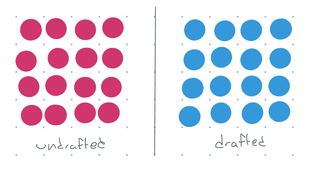
figure 4: red = didn’t serve, blue = served. all undrafted don’t serve, all drafted do serve. each dot represents many people.
But the draft wasn’t that clean. There are people who were drafted but didn’t serve: people who were physically unfit, conscientious objectors, college students, people who moved to Canada to avoid the draft, and so on. There were also people who weren’t drafted but willingly chose to volunteer, because they wanted to serve their country or who strongly agreed with the war. And of course, there are people whose military service was fully determined by the draft: people who wouldn’t have served if undrafted, but served because they were drafted. So instead of the above picture, the population looks something like this.
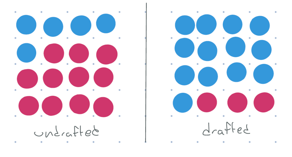
figure 5: red = didn’t serve, blue = served. some undrafted do serve, but more people in the drafted group serve.
So taking the difference of mean earnings between those who were drafted and those who were undrafted won’t be perfect. It won’t get us the causal treatment effect of military service. It’ll be “muddled” because of the fact that there was imperfect compliance. So figuring out the treatment in a straightforward way isn’t so easy.
What I’m going to show below is that it is possible to find a treatment effect from our data: the effect of military service on wages for people compelled to serve only because of the lottery. I’ve tried to make the derivation as clear as possible, but if you’re not interested in it, skip past the equation marked (⋆).
So what can we do? If we draw out the population as above, it’s actually possible for us to see visually the three types of groups talked that we talked about:
- “Always-takers”: people that would have served, no matter what
- “Compliers”: people who served only because they were drafted
- “Never-takers”: people who never would have served in the military
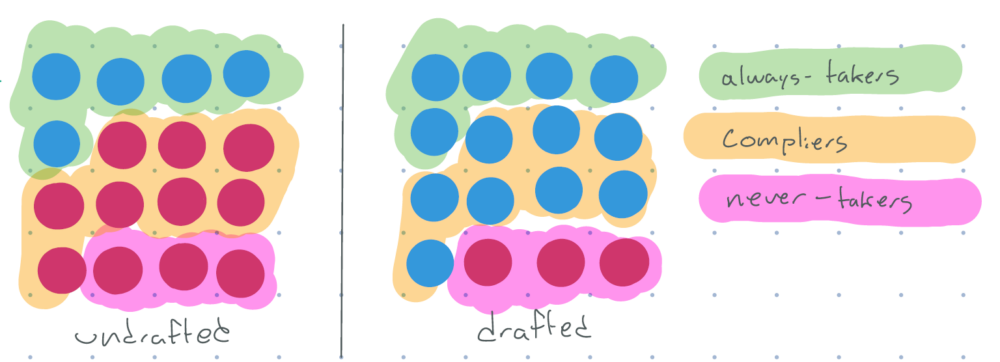
figure 6: red = didn’t serve, blue = served. some undrafted do serve, but more people in the drafted group serve. divided into groups of always-takers, compliers, and never-takers.
Of course, it’s impossible for us to exactly determine who these people are across the whole population, because we don’t observe people’s counterfactual choices. But because the lottery was random, we can say a few things about the average wages for different groups.
- The always-takers who were undrafted are easily identified: they’re the only people who serve when undrafted. Because our assignment was random, the average earnings for this group of people will be (statistically) similar to the average earnings of the always-takers who were drafted.
- Similarly, the drafted never-takers can also be easily identified: they’re the people who were drafted but didn’t serve. Again, we can compute their average earnings, which should be similar to the average earnings for never-takers who weren’t drafted.
Armed with this knowledge, we can use some math (and using the notation that P(⋅) is the fraction of the population who were in some group, i.e., the probability that a randomly chosen individual is in that group) to rewrite the difference in the mean earnings of drafted and non-drafted people as
Mean Earnings of Drafted–Mean Earnings of Undrafted =Mean Earnings of Drafted Always-Takers⋅P(Always-Taker) +Mean Earnings of Drafted Compliers⋅P(Complier) +Mean Earnings of Drafted Never-Takers⋅P(Never-Taker) –Mean Earnings of Undrafted Always-Takers⋅P(Always-Taker) –Mean Earnings of Undrafted Compliers⋅P(Complier) –Mean Earnings of Undrafted Never-Takers⋅P(Never-Taker) =Mean Earnings of Drafted Compliers⋅P(Complier) –Mean Earnings of Undrafted Compliers⋅P(Complier) =P(Complier)(Earnings of Drafted Compliers–Earnings of Undrafted Compliers)
In other words, the difference in means is exactly the fraction of the population that are compliers multiplied by the difference in earnings between compliers who drafted (and thus served) and compliers who weren’t drafted (and so didn’t serve). Note that the second term in the multiplication is exactly the treatment effect that I claimed above: the effect of military service on wages for the people who were compliers! All that we’d need to do is to divide by the fraction of the population that are compliers. That number is easy to find: it’s just the fraction of people who served when drafted, subtracting the fraction of people who served when undrafted.
And so, we can write the following:
Treatment Effect for Compliers=Mean of Drafted – Mean of UndraftedFraction of Drafted who Served – Fraction of Undrafted who Served(⋆)
In this context, it turns out that service in the Vietnam War had no impact on the earnings for compliers who were minorities, while white veterans who were compliers had a 15% decrease in wages compared to those who weren’t drafted. For more details, check out Angrist (1990), “Lifetime Earnings and the Vietnam Era Draft Lottery: Evidence from Social Security Administrative Records”.
The above estimator, (⋆) is an example of an instrumental variables approach (or IV), also used very frequently by applied economists. The thing that affects the denominator (here, the draft), is called an instrument — hence the name. Angrist and Imbens showed that the number computed above is the treatment effect for compliers, called the Local Average Treatment effect (or LATE) — see Imbens and Angrist (1994), “Identification and Estimation of Local Average Treatment Effects”.
There’s a few important assumptions that I made implicitly, without really talking about them:
- (Random Assignment) The draft happened in a way that is completely unrelated to people’s wages or intention to serve. As the draft happened by birthdays, it is almost surely random here.
- (Relevance) The draft impacted some people’s choice to serve in the military. If there was no such impact, the denominator of (⋆) would be 0, which would not be good. So we make this assumption c:
- (Exclusion) The draft only impacted people’s earnings through the channel of making people serve. If it didn’t — say, people weren’t aware that the draft was random, thought that not being drafted was a sign that they weren’t “good enough” for the military, and so took a self-confidence hit, which impacted which jobs they applied to — then being drafted itself would impact wages, and we wouldn’t be able to figure out any sort of treatment effect. The exclusion restriction is not directly testable in most circumstances, and is an assumption we have to make.
- (Monotonicity) There are no “defiers” — people who would have served had they been undrafted, but didn’t serve because they were drafted. It makes sense that very few defiers exist in this context, but there are some types of interventions where you may have defiers. If there are defiers, then we wouldn’t be able to clearly identify the lifetime earnings of always-takers or never-takers.
But — under all of these conditions — we are able to look at data and figure out something deep about the world.
Other such papers using instrumental variables include:
- Angrist and Krueger (1991), “Does Compulsory School Attendance Affect Schooling and Earnings?”, which uses people’s quarter of birth as an instrument to determine the impact of years of (compulsory) school on earnings, since your quarter of birth determines how “early” you can drop out of school.
- Kling (2006), “Incarceration Length, Employment, and Earnings”, using randomly assigned judges to create an IV estimate of how sentencing length impacts later earnings.
When I took AP Micro and Macro, I thought a lot about where the models we were using came from, how “true” they were in reality, and whether we can make better ones. It turns out that this is exactly what empirical economics does: takes some theory that we have, and tries to test it in the world using methods like D-in-D and IV. The seminal work of Card, Angrist, and Imbens helped to kick off the credibility revolution, a movement that has shaped the entire field of economics research today.
And that’s just about it for this blogpost! A lot all at once, yes, but a derivation of Nobel Prize-winning research in just a single blog post. If you’re interested in learning more, The Nobel Foundation actually creates a popular science background (slightly easier to read than this) and also a more scientific background (harder to read than this) that delves much more into the research papers and the methodology. There are also a few other methods that economists use — Randomized Controlled Trials (RCT) and Regression Discontinuity (RD) — to learn about the world, and I encourage you to look into these more if you’re interested.
But for now, this is the end of my quick07 maybe not so quick, this is over 3500 wordsprimer on economics and Nobel Prize-winning research. If this all piqued your interest — then hey, maybe economics is right for you c:
Comments